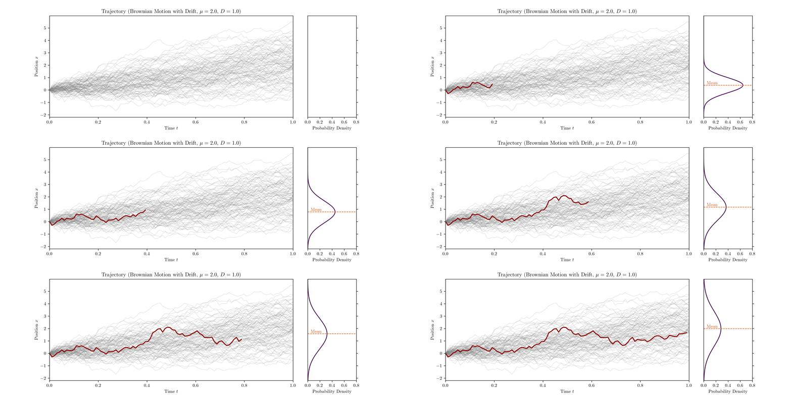
Brownian Stocks
A fun weekend project where I modeled stock prices using Langevin Dynamics.
Langevin Dynamics
When it comes to understanding the dynamics of complex systems, one often encounters the interplay between predictable, deterministic forces and unpredictable, stochastic influences. The most versatile tool to studying these processes is by far Langevin dynamics. We can for example consider a particle in a medium on a trajectory $x(t)$. The particle (e.g., an ion) may obey a deterministic force, such as a potential gradient $-\nabla U(x(t))$. It is thereby exposed to the immediate neighborhood in its environment and thus experiences a damping, frictional force proportional to its velocity: $-\gamma \frac{dx(t)}{dt}$. Finally, the precise movements and individual steps of the particle are subject to some degree of randomness, which may obey certain correlation properties. Langevin dynamics express these factors in terms of Newton’s equation:
\[m \frac{d^2x(t)}{dt^2} = -\gamma \frac{dx(t)}{dt} - \nabla U(x(t)) + \eta(t),\]where $m$ is the mass of the particle, $\gamma$ is a damping (friction) coefficient, and $\eta(t)$ is a stochastic noise term. The latter may for example be modeled as Gaussian white noise. Now, in the case where the damping and fluctuations dominate, for example if the particle mass is very small, we find $m \frac{d^2x(t)}{dt^2} \ll \gamma \frac{dx(t)}{dt}$ and inertia becomes increasingly irrelevant. This is the transition into Brownian motion.
Brownian Motion
Brownian motion refers to an edge case in Langevin dynamics, where the influence of inertia is negligible compared to the deterministic and stochastic forces acting on the system. In this overdamped limit, where $m \frac{d^2x(t)}{dt^2} \approx 0$, the Langevin equation reduces to
\[\frac{dx(t)}{dt} = -\frac{1}{\gamma}\,\nabla U(x(t)) + \frac{1}{\gamma}\,\eta(t).\]This is a first-order differential equation in time, which we can formally integrate over a small interval $\Delta t$ to retrieve the displacement $\Delta x$.
The deterministic contribution, $-\frac{1}{\gamma}\,\nabla U(x(t))$, acts as a drift term defining the mean direction of motion. For small or constant gradients, this results in a constant drift $\mu$:
\[\mu = -\frac{1}{\gamma}\,\nabla U(x(t)).\]The stochastic contribution, $\frac{1}{\gamma}\,\eta(t)$, becomes a stochastic increment as we consider $\eta(t)$ as ideal white noise. This increment is understood as coming from a Wiener process, where the increments $\Delta W$ are drawn from a normal distribution with zero mean and a variance proportional to the time increment $\Delta t$:
\[\Delta W \sim \mathcal{N}(0, \Delta t).\]Worth noting, this is just one approach of a broader class of models known as Lévy processes, which differ in their assumption of the distribution of increments.
We can now describe the trajectory $x(t)$ by the stochastic differential equation
\[dx(t) = \mu \, dt + \sigma \, dW(t).\]$\mu$ is a constant drift term that accounts for any directional bias the particle may experience, for example from an electric field, and $\sigma$ quantifies the intensity of the fluctuations. $dW(t)$ represents the increments of the Wiener process.
Considering an ensemble of particles, $\mu$ essentially determines the mean displacement around which the ensemble spreads over time. We also know from statistical mechanics and the Green–Kubo relations that the mean square displacement (in 1D) is related to the diffusion constant $D$ via
\[\langle (x(t)-x(0))^2 \rangle = 2 D t.\]Finally, it follows from the Itô isometry that
\[D = \frac{\sigma^2}{2},\]which connects the microscopic fluctuations of the system to the macroscopic diffusion constant.

Black–Scholes Model
The principles of Brownian motion extend naturally into the realm of asset pricing and form the backbone of the Black–Scholes model. However, rather than having additive increments that allow for negative values in the trajectory, we here consider the process in a multiplicative manner. The resulting process is known as geometric Brownian motion (GBM). For an asset price $S(t)$, the differential equation is then
\[dS(t) = \mu \, S(t) \, dt + \sigma \, S(t) \, dW(t),\]where the $S(t)$ in both the drift and diffusion term account for the proportional nature of price changes and keep the price positive. The drift parameter $\mu$ represents an expected return rate, while $\sigma$ is the volatility of the asset.
While this model reflects more closely the multiplicative changes in financial markets, this is at the expense of analytical convenience.
Instead of working with the raw returns, it is thus convenient to introduce log returns. Not only because this re-introduces an additive framework (multiplicative processes become additive in log space), but also because evidence suggests that log returns tend to be more normally distributed than raw returns, aligning better with the model’s fundamental assumptions. By applying Itô’s lemma, the stochastic differential equation for the log price becomes
\[d\ln S(t) = \left(\mu - \frac{\sigma^2}{2}\right) dt + \sigma\, dW(t).\]This equation is now again equivalent to simple Brownian motion from the very beginning, except that the drift term is modified by what is known as the Itô correction.
We can now apply this model to data from yfinance, where it’s worth underlining that this model relies on a few coarse assumptions beyond normally distributed log returns. We also assume, among others, that the volatility remains constant and that trading involves no transaction costs (friction-less…). The normal distribution provides us the corresponding drift and diffusion constants. We can use this in turn to model the “theoretical” time series by a Markov model. In each iteration, we update the price according to

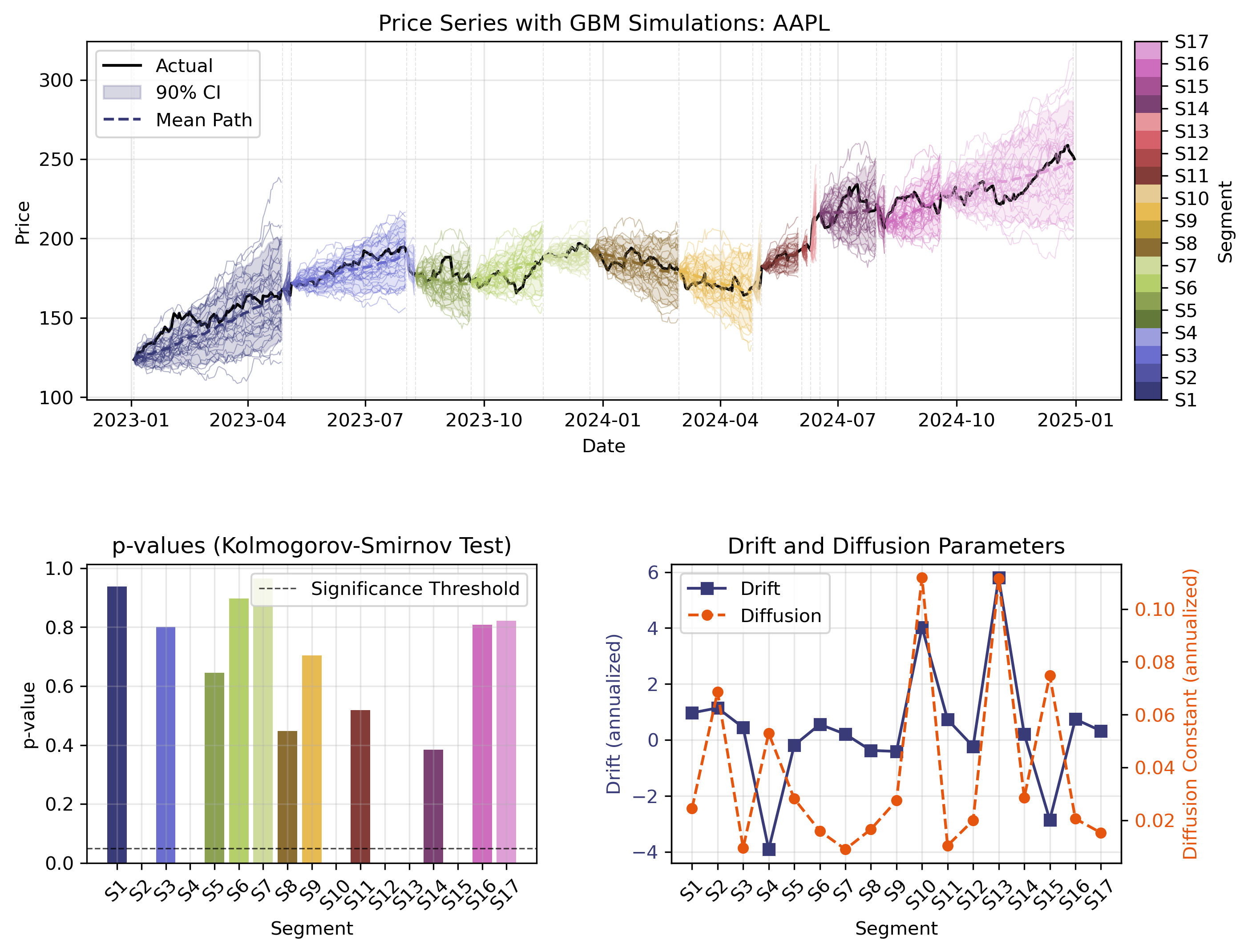
Evidently, the assumption of geometric Brownian motion performs rather poorly in reproducing the stock’s trajectory over such a long time span. This is not surprising, given that GBM assumes constant drift and diffusion parameters over the entire time period. To address this limitation, we can segment the time series into periods where GBM might hold more closely.

To this end, we can use a PELT (Pruned Exact Linear Time) algorithm, which identifies multiple change points in the time series by minimizing a cost function. For each segment, we validate the GBM assumptions using the Kolmogorov-Smirnov (KS) test, which compares the empirical distribution of log returns to a normal distribution. We can then also calculate physical parameters such as drift $(μ)$, volatility $(σ)$, and diffusion constant $(D = \frac{σ^2}{2})$.
We perform Monte Carlo simulations for each segment with 100 paths each, providing the confidence intervals to quantify our uncertainty. Evidently, this approach provides a much better fit to the actual price trajectory.